A martingale approach to detect changes in histograms
December 15, 2016
If a user has opted into submitting performance data to Mozilla, the Telemetry system will collect various measures of Firefox performance, hardware, usage and customizations and submit it to Mozilla. Telemetry histograms are the preferred way to track numeric measurements such as timings.
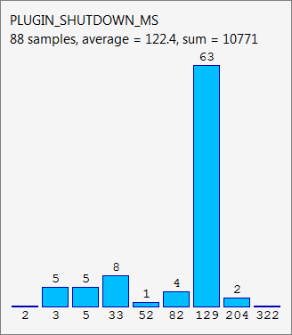
The histogram below is taken from Firefox’s about:telemetry page. It shows a histogram used for tracking plugin shutdown times and the data collected over a single Firefox session. The timing data is grouped into buckets where the height of the blue bars represents the number of items in each bucket. The tallest bar, for example, indicates that there were 63 plugin shutdowns lasting between 129 ms and 204 ms.
The previous metric is just one of the many the Firefox browser collects and sends over to our pipeline, which aggregates metrics by build and submission date and makes the roll ups available through the telemetry.js v2 API as time series:
 Detecting changes over time is crucial to alert developers when a build regressed a performance measure. There is an ad-hoc system in place at the moment but it’s hard to tune and adapt to new measurement types.
Individual histograms can be represented as vectors. What we ultimately want to test is if a sequence of vectors, i.e. a time series for a particular measure, is independent and identically distributed. As traditional statistical approaches to test this property are inappropriate for high dimensional data we tried to address this problem using martingales.
Martingales?
A martingale is a model of a fair game where knowledge of past events never helps predict the mean of the future winnings and only the current event matters. In particular, a martingale is a sequence of random variables for which, at a particular time in the realized sequence, the expectation of the next value in the sequence is equal to the present observed value even given knowledge of all prior observed values.
Before we describe how a martingale can be used to detect changes in time series, we introduce the concept of strangeness measure to assess how much an observation differs from other ones. Say we have a set of vectors and we want to determine how different a new vector is from . One way to do that is to compute the average vector from and take the euclidean distance of from . The euclidean distance acts as a strangeness measure in this case.
The martingale change detection algorithm proceeds in two steps. Observations are presented one by one in an online fashion. For each new observation , its strangeness score is determined and consequently its p-value computed given the scores of past observations:
where is a random number from . It can be shown that if all observations are i.i.d. then the p-values are uniformly distributed in .
In the second step a family of martingales is introduced, indexed by , and referred to as the randomized power martingale:
Where the s are the p-values discussed above, with the initial martingale . If and when the martingale grows larger than a set threshold , the assumption that there is no change in the time series can be rejected based on Doob’s inequality:
This inequality means that it is unlikely for any to have a high value.
Implementation
The implementation is relatively straightforward but we had to tweak it to adapt it to our use case. To highlight the salient points we will use only a few measurements to do so but bear in mind that they apply more generally to other measures as well.
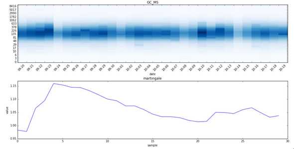
Let’s start by checking how the change detection algorithm, with the cosine distance as strangeness measure, performs on a time series we know didn’t change. GC_MS tracks the time spent running the Javascript garbage collector in ms:
As shown in the plots above, the histogram exhibits a weekly seasonality due to the fact that less data is collected during the weekends. That seasonality can cause the martingale to grow when it really shouldn’t which ultimately could lead to false positives.
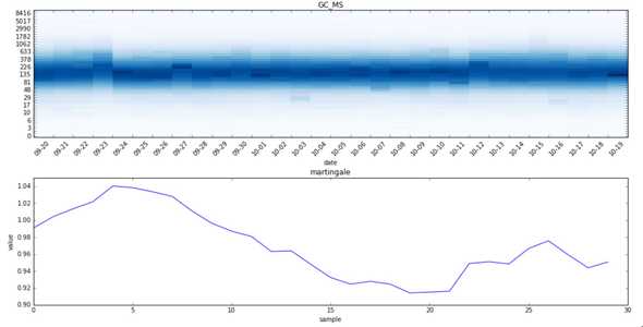
Since we mostly care about the shape of the histogram we will try normalizing the histogram first:
As the plots show, the martingale now grows less than in the previous case as we reduced the noise in the time series by eliminating the seasonality.
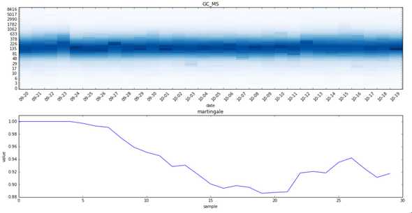
Notice also how the martingale grows initially since it hasn’t seen yet many observations. That can cause to yield a higher number of false positives under some circumstances. To avoid it we will force the martingale to not change for the first points so that the algorithm has a chance to learn how the strangeness distribution looks like.
Now we will test the change detection algorithm on a histogram known to have changed in the given time period.
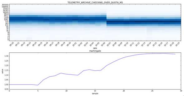
TELEMETRY_ARCHIVE_CHECKING_OVER_QUOTA_MS measures the time in ms it takes to check if the telemetry archive is over-quota:
The heatmap shows clearly that there was a change on the 7th of October. The problem now is that that the martingale doesn’t grow fast enough and tends to stay close to 1 and as such Doob’s inequality is hardly applicable. This is due to the fact that we have only few data points available.
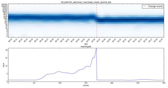
One way to deal with the martingale not growing fast enough is “to cheat” and use spline interpolation to generate more points.
Now we can spot a nice spike in the martingale plot! Note also how the martingale is reset to 1 when it crosses the configurable change threshold which in this case is set to 20.
The proposed algorithm catches many changes that are easily spotted by a human but also some that are debatable. Ideally we want to reduce the number of false positives as much as possible even at the cost of missing some real changes. A high number of false positives could cause developers to loose trust, and ultimately ignore, the detected changes.
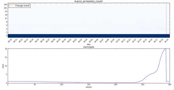
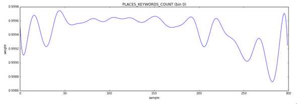
It’s very hard to see any change at all in the heatmap for PLACES_KEYWORDS_COUNT. What’s going on? It appears that bin 0, where most of the distribution is concentrated, is mostly stable until it isn’t; in other words a slight change of that bin can cause the martingale to grow very fast:
One way to deal with the issue is to increase the change threshold which in turn can cause to miss some real changes. A better way to deal with it is to check how the histogram bins are affected before and after a detected change and ignore it if the weight difference is so small that even if it is statistically significant it isn’t practically of relevance.
Without further ado let’s see some other changes caught by the algorithm in the given time period:
Note how the martingale grows slightly around the 3rd of October where there was a temporary change.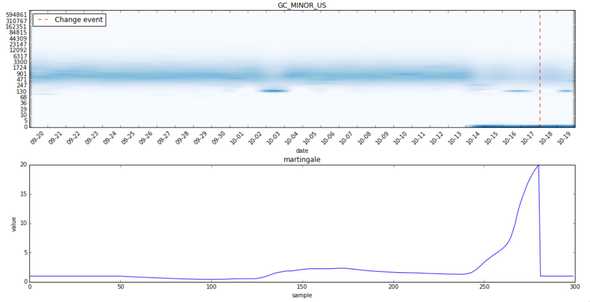
This histogram is rather noisy and we will have to blacklist it.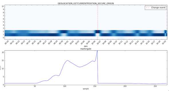
Bins 0 and 1 have been practically inverted on the 6th of October.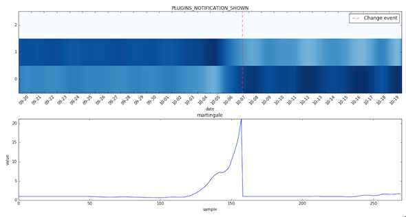
Note how the martingale grew during the first change around the 28th of September and then slowly started decreasing after the time series nearly went back to its original form.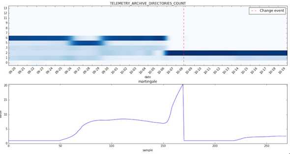
And now a few histograms for which no change was detected:
This histogram is way too noisy and the martingale plot reflects it.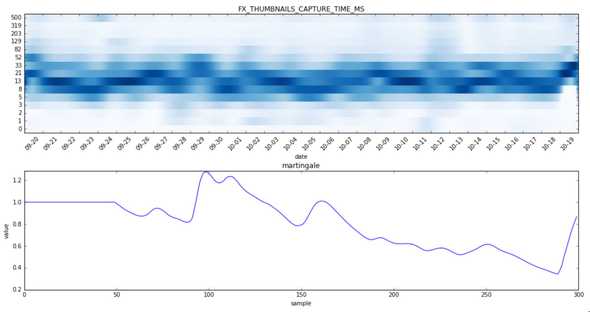
This histogram didn’t change at all.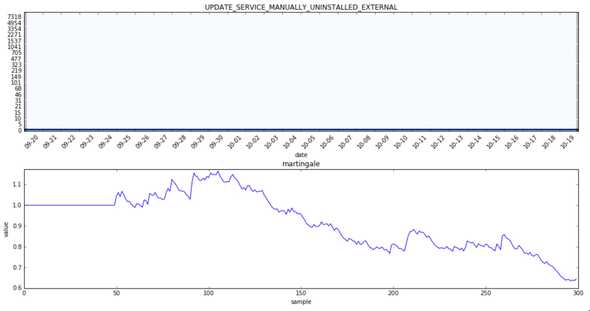
Evaluation
Since our time-series are unlabeled we were forced to evaluate the performance and tune the parameters of our anomaly detection algorithm manually. To do so we used the number of changes found and precision to tune our model as we wanted to catch as many anomalies as possible, but more importantly, keep the number of false positives to a very small number (one digit percentage). Ideally if we had a labelled set of all changes we could just cross-validate our model. Unfortunately that’s not the case though.
We might consider in the future to use Mechanical Turk to label a set of time-series but as it currently stands we don’t have the time to do so ourselves as the number of histograms is extremely high (in the order of several thousands) and labeling anomalies requires not only to look at the data but also to consider known performance regressions/changes of the Firefox browser.
